![]()
AMOVA in R
Resources for conducting population genetic and phylogenetic analyses in the R computing environment are continually improving, and to date several packages have provided functions for estimating phi-statistics and hierarchical patterns of population variance partitioning using AMOVA (analysis of molecular variance; Quattro et al. 1992). The paper for the AMOVA method, penned by population geneticists Joe Quattro, Peter Smouse, and Laurent Excoffier, now has >12,000 citations, making it one of the most used and cited methods of all time in evolutionary genetic analysis; many people continue using this method, including me. What is interesting about recent packages is that they allow us to do AMOVA rather easily on SNP data, and today I’m going to show you some code for conducting AMOVA in R on biallelic SNPs.
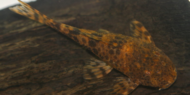 Hypostomus sp. 2; Photo Credit: Pedro P. U. Aquino
I’ll be using an example of SNP sites from ddRAD-seq analyses of Hypostomus suckermouth armored catfishes (sp. 2, pictured at left), that are hierarchically spatially distributed as individuals, within sites (populations), within three drainage basins in central Brazil. We are going to start from SNPs, get the SNPs into R using the packages adegenet (Jombart 2008; Jombart and Ahmed 2011; Jombart et al. 2015) and poppr (Kamvar et al. 2014, 2015), and then conduct some data massaging/prepwork before conducting final AMOVA analyses using the same packages. The analyses will experiment with the effects on AMOVA results of varying the missing data level threshold in poppr’s AMOVA function (i.e. the “cutoff” option within ‘poppr.amova’ function).
Practical
SETUP: Load R packages
First, let’s open R (as of initial writing, I’m using R version 3.3.2 (2016-10-31) – “Sincere Pumpkin Patch”) and set up the workspace by loading adegenet and poppr; let’s also load the APE library just in case we need it. If you don’t have R, then download the latest version for Windows here, and download the latest version for Mac OS X here. If you have R but don’t have the packages, then install them from within R by typing install. packages(“name”) where name is the name of the package.
library(adegenet)
library(poppr) ## Ignore 'OMP parallel support' info...
library(ape)
SETUP: Read in the data
Next, we’ll read in the data and process it (see next code section below). We will start by reading my SNP data into R from a file with an “.str” extension in the current working directory, in which the data are stored in STRUCTURE format. This data file contains a moderate number of SNPs (representing 1 SNP per RAD tag) from central Brazilian Hypostomus suckermouth armored catfish populations, and it was originally output by pyRAD following data assembly and SNP calling. Here, in my case, the data were produced by NGS sequencing on a ddRAD-seq genomic library that included outgroup samples, in order to facilitate downstream phylogenomic analyses. However, we need to make sure that we only do AMOVA on the ingroup data, because we are interested in patterns of hierarchical genetic structure in the focal species, and not in focal species + outgroup. Including outgroup individuals would in fact bias the results. So, we must start by reading in a data file that contains only ingroup Hypostomus individuals, and no outgroup individuals (hence the “noout” code in the file name).
I will do this below using the following four steps: * Step #1: read in the data as a genind object * Step #2: convert the data frame from a genind object to a genclone object using the ‘as.genclone’ function of poppr (note: as.genclone is available as of poppr v2.2.1, but may or may not be available in later versions of the package) * Step #3: read in a hierarchy file * Step #4: recreate the genclone object after specifying the hierarchy to the genind object as the strata.
Here is the code…
Step #1
###### READ STRUCTURE DATA INTO R AS GENIND OBJECT
Hyp.genind.noout = import2genind('hypostomus_noout.str', onerowperind=F, n.ind=40, n.loc=226, row.marknames=NULL, col.lab=1, ask=F)
Step #2
## CONVERT GENIND OBJECT TO A GENCLONE OBJECT
Hyp.genclone.noout = as.genclone(Hyp.genind.noout)
Step #3
The name of my hierarchy file is “Hyp_3hier_ind-pop-drain_assignments.txt” and the first 10 lines of this file looks as follows:
ind pop drain

1 1 6 3

2 2 1 1

3 3 7 1

4 4 7 1

5 5 1 1

6 6 9 3

7 7 10 1

8 8 10 1

9 9 1 1

10 10 10 1
Here is the code for the hierarchy file:
## READ IN HIERARCHY FILE
##--Input a hierarchy file that specifies individual number, population number, and factor/group
##--number. The name of my hierarchy file is "Hyp_3hier_ind-pop-drain_assignments.txt"; I read it in using
##--the 'read.table' function.
Hyp.hier.noout = read.table('Hyp_3hier_ind-pop-drain_NOOUT_assignments.txt', header=T)
Step #4
Now we can add the hierarchy information in one of two ways:
## Example #1:
Hyp.gc.strat.noout = as.genclone(Hyp.genind.noout, strata=Hyp.hier.noout)

## Example #2
strata(Hyp.genind.noout) = Hyp.hier.noout[-1]
pop(Hyp.genind.noout) = c(6, 1, 7, 7, 1, 9, 10, 10, 1, 10, 10, 10, 11, 11, 11, 11, 1, 1, 1, 12, 1, 8, 9, 9, 14, 2, 2, 2, 2, 2, 2, 2, 3, 3, 4, 5, 5, 6, 6, 6)
Hyp.gc.strat.noout = as.genclone(Hyp.genind.noout)
The purpose of showing these steps in this order is to demonstrate that we can easily convert from genind to genclone; however, it is better–in fact, necessary–that we do this for AMOVA while adding information about the hierarchical relationships (population hierarchy) of the dataset. In the last commands, under Step #4 “Example #2”, the individual information is already present in the genind object, we just needed to add the population and hierarchy information.
ANALYSIS: AMOVAs
OK, that’s it for processing! Now, we’re ready to conduct AMOVAs and get some results for our Hypostomus populations. As noted above, we will run separate AMOVA analyses using different cutoff values for missing data. This “cutoff” value sets the level at which missing data will be ignored or modified during calculations. It’s somewhat counterintuitive, but a low value will specify a low missing data threshold and thus identify and remove more sites with missing data from the analysis, leaving potentially many fewer sites for analysis. By comparison, a high cutoff value will result in leaving more sites for analysis, depending on the distribution of missing data in the data frame. In my case, as you’ll see below, a 95% cutoff value removed 0 loci. But let’s see if changing the cutoff value from 30% (analyzing fewer sites) to 95% (analyzing more sites) changes the outcome for the Hypostomus headwater fish system.
Here is the code for doing the AMOVAs and significance tests (to get p-values):
## AMOVA TESTS (not including outgroup individuals)
## Do Hyp AMOVA with 0.3 (30%) missing data cutoff (leaves fewer sites):
Hyp.drain.amova.res = poppr.amova(Hyp.gc.strat.noout, ~drain/pop, cutoff=0.3)
Hyp.drain.amova.res
Hyp.drain.amova.test = randtest(Hyp.drain.amova.res)
str(Hyp.drain.amova.test)
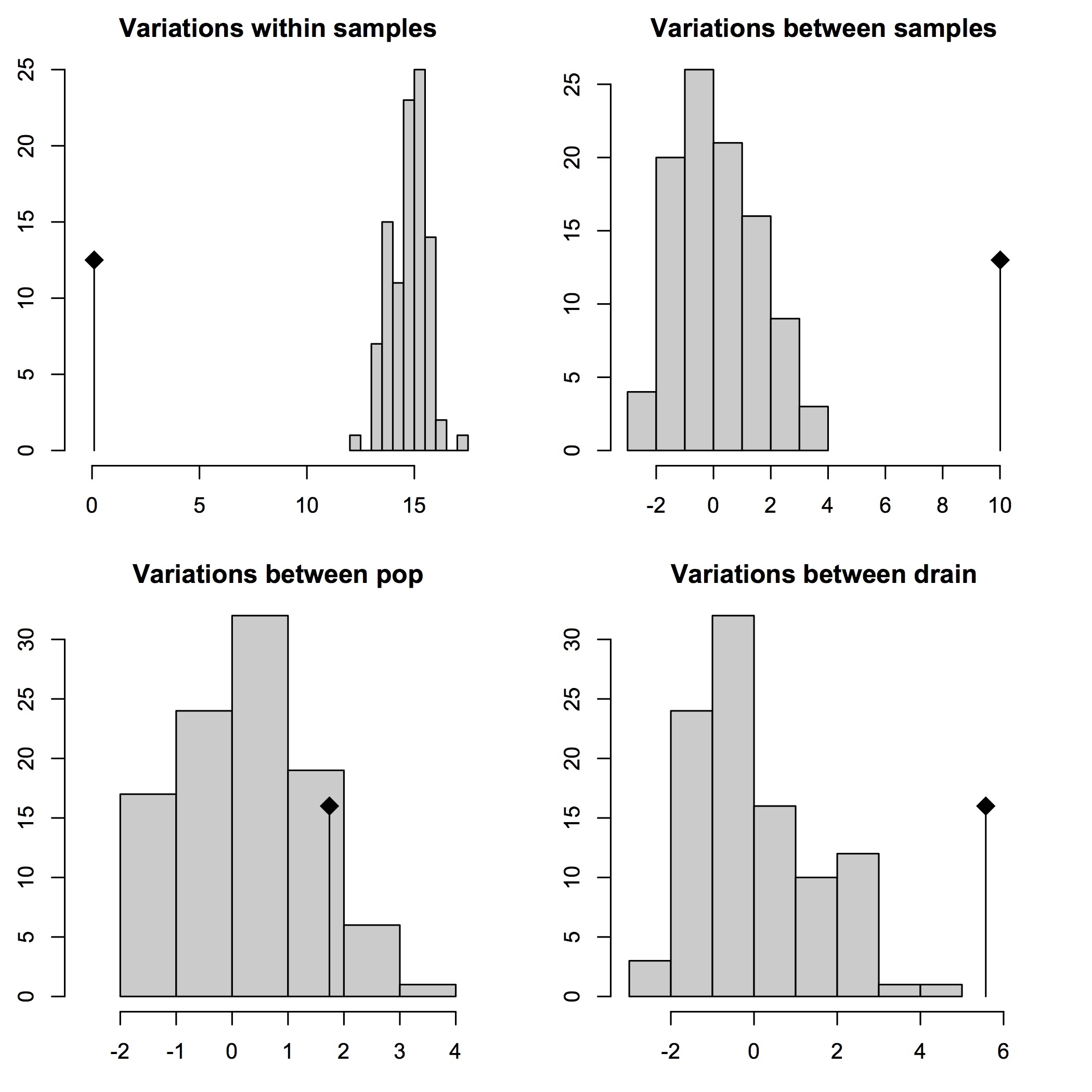
plot(Hyp.drain.amova.test)
Hyp.drain.amova.test
## Do Hyp AMOVA with all the data, by using an 0.95 (95%) missing data cutoff (leaves more sites):
Hyp.drain.amova.res.95 = poppr.amova(Hyp.gc.strat.noout, ~drain/pop, cutoff=0.95)
Hyp.drain.amova.res.95
Hyp.drain.amova.test.95 = randtest(Hyp.drain.amova.res.95)
str(Hyp.drain.amova.test.95)
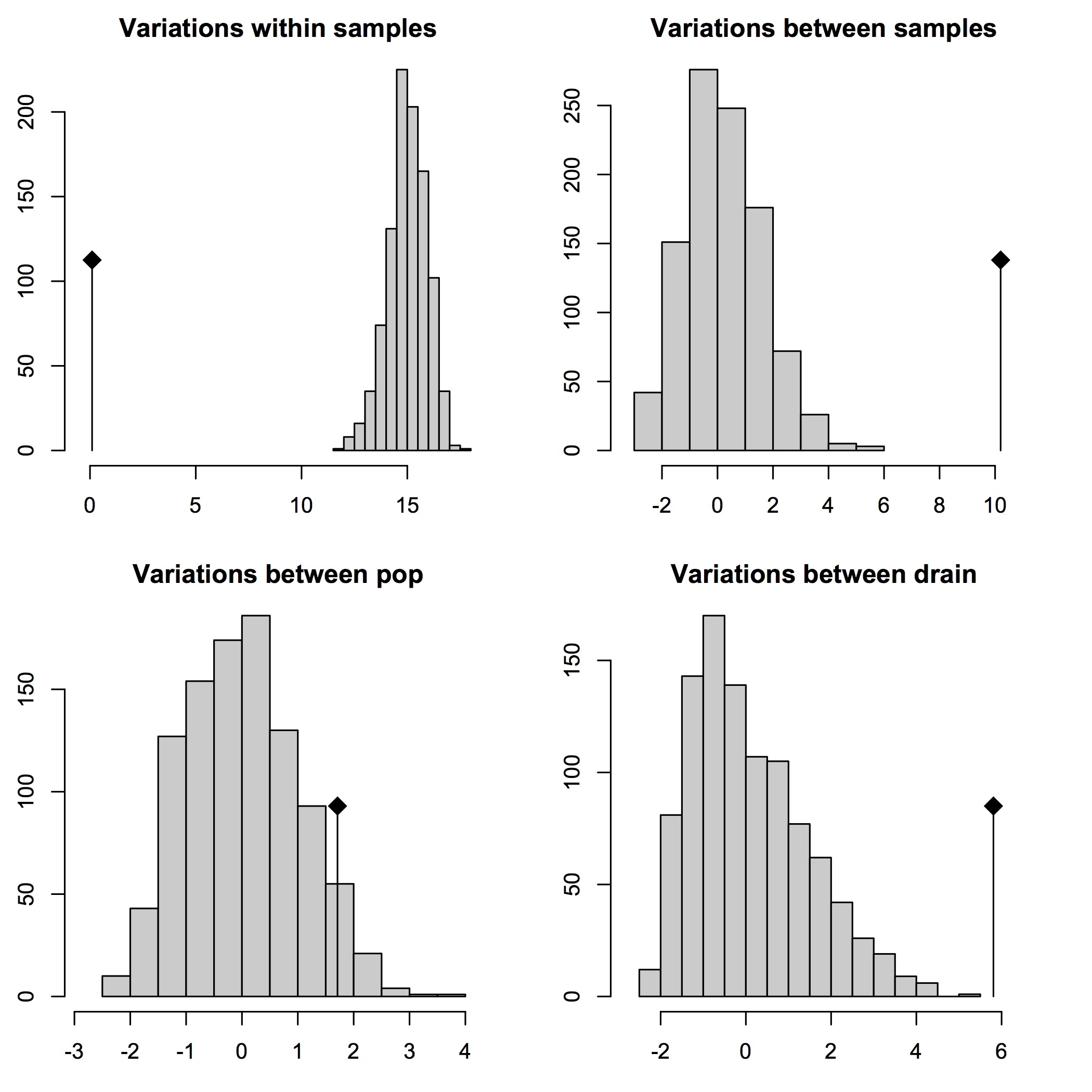
plot(Hyp.drain.amova.test.95)
Hyp.drain.amova.test.95
When I ran the above code and called R to print the basic AMOVA results to screen for both models (by typing “Hyp.drain.amova.res” or “Hip.drain.amova.res.95” and then pressing Enter), the basic pattern of change in the number of sites in the analyses was as follows: 338 of the 3,829 total SNPs in the dataset were removed due to having 30% missing data (or more, but this is very unlikely; see below) during the 30% cutoff analysis, and 0 SNPs were removed due to missing data in the 95% cutoff analysis (results not shown).
RESULTS!
Now, let’s look at the results of variance partitioning, as well as the significance of the variation within and between groups, as they would be pictured in the R console (GUI) window:
30% cutoff AMOVA results
## 30% cutoff covariance and Phi-statistics results:
...
$componentsofcovariance
                                             Sigma          %
Variations  Between drain               5.10788445  27.509734
Variations  Between pop Within drain    3.42570578  18.449958
Variations  Between samples Within pop  9.93798617  53.523403
Variations  Within samples              0.09597662   0.516905
Total variations                       18.56755302 100.000000

$statphi
                        Phi
Phi-samples-total 0.9948309
Phi-samples-pop   0.9904348
Phi-pop-drain     0.2545164
Phi-drain-total   0.2750973
## 30% cutoff significance test results:
                        Test        Obs    Std.Obs   Alter Pvalue
1  Variations within samples 0.09597662 -15.327787    less   0.01
2 Variations between samples 9.93798617   6.716293 greater   0.01
3     Variations between pop 3.42570578   2.566409 greater   0.02
4   Variations between drain 5.10788445   4.266484    less   1.00
95% cutoff AMOVA results
## 95% cutoff covariance and Phi-statistics results:
...
$componentsofcovariance
                                             Sigma          %
Variations  Between drain               5.10788445  27.509734
Variations  Between pop Within drain    3.42570578  18.449958
Variations  Between samples Within pop  9.93798617  53.523403
Variations  Within samples              0.09597662   0.516905
Total variations                       18.56755302 100.000000

$statphi
                        Phi
Phi-samples-total 0.9948309
Phi-samples-pop   0.9904348
Phi-pop-drain     0.2545164
Phi-drain-total   0.2750973

## 95% cutoff significance test results:
                        Test        Obs    Std.Obs   Alter Pvalue
1  Variations within samples 0.09597662 -16.617535    less   0.01
2 Variations between samples 9.93798617   7.826314 greater   0.01
3     Variations between pop 3.42570578   3.095911 greater   0.01
4   Variations between drain 5.10788445   3.725359    less   1.00
Conclusions
Overall, these results showcase two main findings.
First, we can reject the null hypothesis of panmixia in favor of significant genetic structuring within and between individuals, as well as at the level of populations within drainages (p < 0.05), with ~99.5% of the variance in the data being present at these three levels. However, there is support for random gene flow between populations in different drainages, and in large part this is due to the fact the the genetic populations (e.g. admixture groups from fastSTRUCTURE) or “clades” (inferred from phylogenomic analyses using maximum likelihood) in the sample occur in multiple drainage basins.
Second, the data are sufficient in number and variability so that AMOVAs on these data are robust to up to 30% (and above) missing data per locus. This makes sense, given that, in pyRAD, these data were stringently filtered so that each RAD tag would contain no more than 30% missing data.
I hope that you have enjoyed doing AMOVA with me! Also, I hope this helps you conduct AMOVA on your phylogeographic or population genomic dataset, in the R environment. Cheers,
~J
References
Excoffier L, Smouse PE, Quattro JM (1992) Analysis of molecular variance inferred from metric distances among DNA haplotypes: application to human mitochondrial DNA restriction data. Genetics, 131(2), 479-491.
Jombart T (2008). adegenet: a R package for the multivariate analysis of genetic markers. Bioinformatics, 24(11), 1403-1405.
Jombart T, Ahmed I (2011) adegenet 1.3-1: new tools for the analysis of genome-wide SNP data. Bioinformatics, 27(21), 3070-3071.
Jombart T, Collins C (2015) A tutorial for discriminant analysis of principal components (DAPC) using adegenet 2.0.0. Imp Coll London-MRC Cent Outbreak Anal Model, 43.
Kamvar ZN, Tabima JF, Grünwald NJ (2014) Poppr: an R package for genetic analysis of populations with clonal, partially clonal, and/or sexual reproduction. PeerJ, 2, e281. doi:10.7717/peerj.281
Kamvar ZN, Brooks JC and Grünwald NJ (2015) Novel R tools for analysis of genome-wide population genetic data with emphasis on clonality. Frontiers in Genetics, 6, 208. doi:10.3389/fgene.2015.00208