Background
In a previous blog post, which has received quite a bit of attention, I detailed how to get “off to a good start” by generating a starting tree for your BEAST analyses. The goal was to work from a tree with branch lengths in units of substitutions per site and to finish with an ultrametric, time-calibrated tree topology with node ages matching calibration points (e.g. fossil ages) you intended to use in BEAST. However, that post was based on things I was doing in 2012, and that were acceptable then, like using ape’s now-deprecated “chronopl” subroutine to do something similar to penalized likelihood (PL; Sanderson, 2002), which is implemented in its fullest form in the r8s software (which, as of this writing, Michael Sanderson stopped updating a couple of years ago at version 1.8). Since that time, Emmanuel Paradis has updated the ape R package to use a new function, “chronos”, for molecular dating on trees using PL and maximum-likelihood. As a result, the goal of this post is to describe how you can use chronos to calibrate the branches of a tree to scale or time units using PL in a way that is more accurate and more sophisticated than what was previously a la mode using chronopl.
So, we’ll again be getting “off to a good start” for BEAST analyses, only this time using more up-to-date methods that I have been having success with now for a year or so.
Go to R…
Just like in the original post on this topic, we’ll want to begin with a standard maximum-likelihood tree, or Bayesian consensus tree, from our data. Once you have generated this “starting tree,” we will then get to work in R in the usual way, by specifying the working directory, loading ape, and inputting our tree.
##Open R, then...
## Specify working directory and load ape:
setwd('~/path/to/working/directory')
library(ape)
#
## Read newick format tree file, like this:
fishtree = read.newick(file='fishes.tre')
## or this:
fishtree = read.tree(file='fishes.tre')
Running chronos in R
OK with the preliminaries; now that that’s taken care of, we’re set up and ready to move forward and run chronos on our starting tree in R. Next, we need to make sure we understand what chronos can do. The chronos function has the following usage:
chronos(phy, lambda = 1, model = 'correlated', quiet = FALSE, calibration = makeChronosCalib(phy), control = chronos.control())
Here, phy is the phylogenetic starting tree, which of course you can name whatever you want; like other trees in ape and other phylogenetics R packages, this is an object of class “phylo”. The lambda argument is for the rate-smoothing parameter for the PL method of Sanderson, which ranges from 0 (indicating no roughness penalty, or that much rate variation is permitted) to 1 (indicating complete smoothing, and actually resulting in a strict clock). The default model also assumes that rates of branch evolution are correlated with one another, so that rate heterogeneity is not accounted for (simplifying assumption; model argument). However, the options for model are “correlated”, “relaxed”, or “discrete,” so you can specify a relaxed-clock model or a discrete rates model as well. The calibration argument points to a “makeChronosCalib” part of the string, which is a tool for preparing data frames containing the one or more calibrations you want to employ. And the control argument part of this is pointing to “chronos.control,” another tool that holds a set of parameters you want chronos to use.
So, in light of the above, it turns out you have several (at least 4) options when using chronos:
- You can put everything into one chronos string and make a new tree (make a treename get the results of calling chronos);
- use makeChronosCalib first to pass calibration information to an object, either passively or in an interactive mode (cool), and then run chronos while simply calling on the corresponding calibration object, and this will give you a new tree;
- or, you could fill chronos.control to first specify important parameter settings, then run Option #1 or Option #2 as usual while calling the corresponding control object, all to get a new tree;
- or, you could do everything including a chronos.control setting in one chronos string.
Four ways of doing a simple example
Here are examples of each of the above options, assuming we have the treefile input above and we are interested in using one fossil calibration ranging between 17-14 Ma (million years ago), which we want to place on node 156 of our phylogeny. Because our tree file is large and the data are non-clocklike, we will use a relaxed clock model, except in the 3rd and 4th examples we will use a special tweak to run a strict clock model. We will also specify the bounds of our calibration to be ‘hard’ rather than ‘soft’ bounds (though this appears it may be unused in the current version of ape, so not sure about that). The output trees will be named timetreex, where x = {1,2,3,4}, corresponding to the above set {Option #1, Option #2, Option #3, Option #4}.
## Option #1:
timetree1 = chronos(fishtree, lambda = 0, model = 'relaxed', quiet = FALSE, calibration = makeChronosCalib(fishtree, node = '156', age.min = 14, age.max = 17, interactive = FALSE, soft.bounds = FALSE))
## Option #2:
abs_calib1 = makeChronosCalib(fishtree, node = '156', age.min = 14, age.max = 17, interactive = FALSE, soft.bounds = FALSE)
timetree2 <- chronos(fishtree, lambda = 0, model = 'relaxed', calibration = abs_calib1)
## Option #3 (making it a strict clock run by specifying a single rate category, and a discrete model):
strict_ctrl = chronos.control(nb.rate.cat = 1)
timetree1 = chronos(fishtree, model = 'discrete', calibration = makeChronosCalib(fishtree, node = '156', age.min = 14, age.max = 17, interactive = FALSE, soft.bounds = FALSE), control = strict_ctrl)
## Option #4:
timetree1 = chronos(fishtree, model = 'discrete', calibration = makeChronosCalib(fishtree, node = '156', age.min = 14, age.max = 17, interactive = FALSE, soft.bounds = FALSE), control = chronos.control(nb.rate.cat = 1))
“What if I have multiple calibration points?”
Glad you asked! This will be a common issue, but fortunately it is also easily dealt with using chronos. Here, the solution is to run makeChronosCalib in interactive mode, which you indicate by specifying the logical argument “interactive = TRUE” instead of the default “FALSE” value. Under the interactive mode, a quartz window will display your tree, and you will then be given the opportunity to repeat the following procedure as many times as you like: 1) select a node, 2) give the minimum age for the node at the keyboard, and 3) give the maximum age for the node at the keyboard. To stop at any time, for example if you accidentally click on the wrong node, simply right click in the quartz window (or do control + click on mac). You can also fix mistakes using fix(cal).
Below are code and screenshots of an example where I used the interactive mode to place three calibration points on a phylogeny of poeciliid fishes. Note that in the above code for options #1-4, I already knew which node to place the calibration point on. You will always need this information to tell chronos which nodes get which calibrations. So, make sure that you have identified the nodes of interest and organized the data for the corresponding calibrations before you run interactive mode. To get the number for a given node that any two taxa in a tree of object class “phylo” (e.g. named “phy”) trace back to, simply run the following code:
mrca(phy)['taxon_name_1', 'taxon_name_2']
This will return the node number, and you’ll need to do this for each node you want to calibrate before proceeding. After you have this information, calibrating multiple nodes is easy. Simply run makeChronosCalib in interactive mode, and add the lower (“youngest age”) and upper (“oldest age”) values for each calibration, like this:
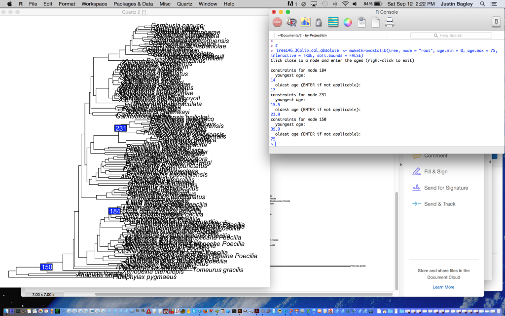
And when you’re done, right clicking will cause the greater than symbol to appear below where you entered your calibration points, signifying the function is closed and R is ready to receive the next line of code.
IMPORTANT: The interactive mode steps I’ve just gone through only place the calibration information inside the calibration object (e.g. in my case, “tree146_3Calib_cal_absolute”). So, this is analogous to using interactive mode in the first step of “Option #2” above. Thus, don’t forget that after doing this you still need to run chronos while referencing your calibration object after the “calibration” flag (like in Option #2 step 2 above). The steps that are missing from my example are:
## Making my 3-calibration time tree:
tree146_3Calib_chronogram <- chronos(tree, lambda = 0, model = 'relaxed', calibration = tree146_3Calib_cal_absolute)
## Plotting the new time tree:
plot.phylo(tree146_3Calib_chronogram, type = 'phylogram', use.edge.length=TRUE, font=3, cex=0.2, no.margin=TRUE)
“What’s the quickest, dirtiest way to get an ultrametric tree using chronos?”
This is also easy. The fastest way to use chronos to go from a non-ultrametric tree to a nice ultrametric tree, without needing to even think about possible calibration points or clock models, is to give chronos no information at all. Just use the chronos defaults, which means a correlated rate model, and only tell chronos which tree to run on, like this:
timetree = chronos(fishtree)
Another way to get a tree quickly is to ask chronos to build a tree to a relative scale. You can accomplish this by first making a relative chronos calibration to scale the length of the tree to 1 by specifying an exact age of 1 for the root, then running chronos to make the relative time tree. Here is an example specifying a relative scale to a total depth of 1, then creating the branch lengths using a relaxed clock PL model with no rate smoothing.
real_calib1 = makeChronosCalib(fishtree, node = 'root', age.min = 1, age.max = 1, interactive = FALSE, soft.bounds = FALSE)
timetree2 = chronos(fishtree, lambda = 0, model = 'relaxed', calibration = rel_calib1)
Conclusion
I’ve shown that chronos provides a flexible means of obtaining time-calibrated branch lengths using penalized likelihood (Sanderson, 2002) over absolute or relative time. So now, using the info above, you should be able to go run the chronos function and make nice input trees for BEAST that will fit your calibrations (or at least be ultrametric)! However, remember you’ll need to write the resulting chronograms to file using something like the write.tree function (usage: write.tree(tree, file="filename")), then you’ll have your tree in newick format that can be supplied to BEAST.
An important difference between chronopl and chronos is that in chronos you cannot simply combine (i.e. concatenate using the “c” combine function, for example c(x, y, ...)) different node numbers and calibration dates to specify multiple calibration points, as could be done using chronopl. This is a good thing though, because Emmanuel has replaced the need to concatenate data with the interactive mode discussed above, and if you try it I’m sure you’ll like it. Just make sure to resize the window, or find a screen large enough to easily visualize the nodes, if you have a very large tree! I say this because the taxon names wind up being really big in the interactive mode window, making it difficult to see the tip taxa and more distal nodes of the tree.
~J
References
Sanderson, M.J. 2002. Estimating absolute rates of molecular evolution and divergence times: a penalized likelihood approach. Mol. Biol. Evol. 19, 101-109.
**Additional ape info: **
http://www.inside-r.org/packages/cran/ape/